5 Join Methods

1. What Join Methods Are

Getting rows with the access methods discussed in the previous chapters is only part of the job. We also need to combine row sets.

A join method is an algorithm for combining two row sets. PostgreSQL uses these algorithms not only to implement SQL JOIN operations, but also for other SQL constructs, such as EXISTS. There are two separate levels: an SQL join is a logical operation that defines which rows belong in the result; a join method is one possible physical algorithm for producing that result efficiently.

We often say that PostgreSQL joins tables. This is convenient shorthand, but the executor actually joins row sets. A row set may come directly from a table through an access method, or it may be the result of another join, aggregation, subquery, or other plan subtree.

Joins are binary: each join node combines two inputs. For ordinary inner joins, the order in which several relations are joined often does not change the logical result, but it can change performance dramatically. The order of the two inputs to one physical join can matter as well.

PostgreSQL has three main join methods: nested loop, hash join, and merge join.

2. Nested Loop Join

The basic nested-loop algorithm is simple: for each row from one input, scan the other input and return the matching rows. Conceptually, it is two nested loops, hence the name.

The first input is conventionally called the outer input; the second is the inner input. A nested loop becomes especially attractive when PostgreSQL can use values from the current outer row to perform a cheap lookup in the inner input. An index is the classic example. If the inner side has to be scanned from beginning to end for every outer row, the same unrelated rows may be examined many times.

For very small inputs, even a repeated scan may still be cheap. Here is a typical nested-loop plan for a small result. We find the segments belonging to two tickets:

EXPLAIN (costs off) SELECT *
FROM tickets t
JOIN segments tf ON tf.ticket_no = t.ticket_no
WHERE t.ticket_no IN ('0005432312163','0005432312164');
                         QUERY PLAN
------------------------------------------------------------
 Nested Loop
   -> Index Scan using tickets_pkey on tickets t
       Index Cond: (ticket_no = ANY ('{0005432312163,000...
   -> Index Scan using segments_pkey on segments tf
       Index Cond: (ticket_no = t.ticket_no)
(5 rows)

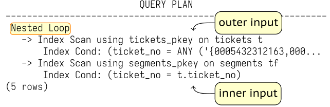
This is a parameterized nested loop. The outer Index Scan produces a ticket row. The value of t.ticket_no from that row becomes a parameter of the inner Index Scan on segments. On each iteration, the inner lookup is effectively performed with a condition of the form ticket_no = constant.

The process continues until the outer input is exhausted.

Now consider another nested loop. We list airplanes whose range is sufficient for two required distances:

EXPLAIN (costs off) SELECT *
FROM ( VALUES (1000), (10000) ) d(range)
JOIN airplanes a ON a.range >= d.range;
                   QUERY PLAN
-------------------------------------------------
 Nested Loop
   Join Filter: (ml.range >= "*VALUES*".column1)
   -> Seq Scan on airplanes_data ml
   -> Materialize
       -> Values Scan on "*VALUES*"
(5 rows)

This join is not parameterized. The inner input does not have an access condition derived from the current outer row. Instead, the inner row set is read repeatedly and the pair is checked by Join Filter. Materialize keeps the tiny VALUES result available for repeated scans, so PostgreSQL does not reconstruct it from scratch on every iteration. Conceptually, this is a Cartesian product followed by filtering.

A nested loop does not require an equality condition. It can implement essentially any join predicate that PostgreSQL can evaluate.

Memoize

If a parameterized inner lookup is executed many times with the same parameter values, repeatedly doing the same work is wasteful. PostgreSQL can cache the results in a Memoize node placed above the inner plan.

If the planner’s estimates incorrectly suggest that memoization is useful, it can be disabled with enable_memoize = off.

Consider a join between routes and airports:

EXPLAIN (analyze, costs off, timing off, buffers off)
SELECT * FROM routes r
 JOIN airports a ON a.airport_code = r.departure_airport
WHERE r.departure_airport in ('BOM', 'SVO');
                         QUERY PLAN
------------------------------------------------------------
 Nested Loop (actual rows=108.00 loops=1)
   -> Bitmap Heap Scan on routes r (actual rows=108.00 l...
       Recheck Cond: (departure_airport = ANY
       ('{BOM,SVO}'::bpchar[]))
       Heap Blocks: exact=33
       -> Bitmap Index Scan on routes_departure_airport_...
           Index Cond: (departure_airport = ANY
           ('{BOM,SVO}'::bpchar[]))
           Index Searches: 2
   -> Memoize (actual rows=1.00 loops=108)
       Cache Key: r.departure_airport
       Cache Mode: logical
       Hits: 106  Misses: 2  Evictions: 0  Overflows: 0
       Memory Usage: 1kB
       -> Index Scan using airports_data_pkey on airport...
           Index Cond: (airport_code =
           r.departure_airport)
           Index Searches: 2
(18 rows)

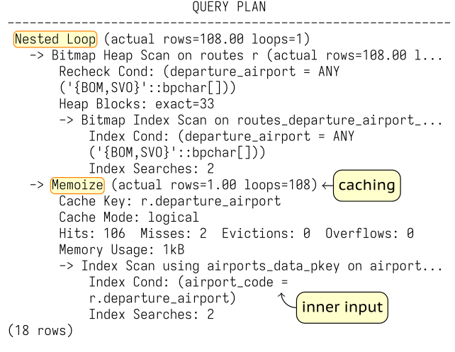
The example is deliberately chosen so that only two distinct parameter values reach the inner side: BOM and SVO.

The first lookup for each value is a cache miss: Misses: 2.

The remaining 106 lookups are served from the cache: Hits: 106.

No entries had to be evicted (Evictions: 0), no cached result overflowed its space (Overflows: 0), and the cache used only 1 kB.

Internally, the cache is keyed by the parameter values of the inner scan. If the outer side repeats the same keys, Memoize can turn repeated inner scans into cheap cache lookups.

Execution Cost

A good first approximation is $N \times \operatorname{cost}(\text{inner probe})$, where N is the number of outer rows. If the inner side is rescanned completely and contains about M rows, this becomes the familiar $O(N \times M)$ comparison pattern.

For a parameterized nested loop, however, the cost of one inner probe may be much smaller than scanning M rows. A unique B-tree lookup, for example, can find at most one matching row after a short tree descent. Repeated probes may also benefit from caching or Memoize.

Nested loop join is effective when the outer input is small and rows of the inner input can be accessed cheaply. In particular, this method, combined with index access, is typical of OLTP queries that need to return a small number of rows very quickly.

Nested Loop in Parallel Plans

Nested loop can participate in a parallel plan.

The outer row set is scanned by several worker processes in parallel. Each worker receives some outer rows and performs the corresponding inner scans independently.

Find tickets associated with inexpensive segments:

EXPLAIN (costs off)
SELECT t.ticket_no, s.price
FROM tickets t
  JOIN segments s ON s.ticket_no = t.ticket_no
WHERE s.price < 1000;

                        QUERY PLAN
----------------------------------------------------------
 Gather
   Workers Planned: 2
   -> Nested Loop
       -> Parallel Seq Scan on segments s
           Filter: (price < '1000'::numeric)
       -> Index Only Scan using tickets_pkey on tickets t
           Index Cond: (ticket_no = s.ticket_no)
(7 rows)

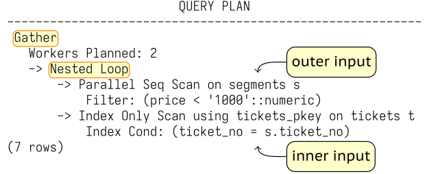
Each participating process scans part of segments. For every qualifying segment it performs its own index-only lookup in tickets. The inner side is not automatically shared just because the outer scan is parallel; each process executes the inner plan for the outer rows assigned to it.

3. Hash Join

Single-Batch Hash Join

In the build phase PostgreSQL reads the inner rows and computes hash values from the join keys.

The in-memory hash table stores the data needed later by the join: the hash value and the projected inner-row data required by the join or by nodes above it.

The memory budget for a hash operation is based on work_mem × hash_mem_multiplier.

For a serial hash join, the best case is that the complete hash table fits in that budget. In that case EXPLAIN ANALYZE reports Batches: 1.

In the probe phase, PostgreSQL reads the outer input sequentially. For each outer row it computes the corresponding hash value, locates the candidate bucket, and then checks the actual join condition.

Checking the hash code alone is not enough. First, not every join condition in the query can be used by a hash join: because a hash function does not preserve value order, hash joins support only equijoins. Second, collisions are possible, when different values receive the same hash code. The probability is small, but it cannot be ruled out.

In the following example large portions of both inputs are needed, so a hash join is a natural choice:

EXPLAIN (costs off)
SELECT *
FROM airplanes a
  JOIN seats s ON a.airplane_code = s.airplane_code;
                    QUERY PLAN
---------------------------------------------------
 Hash Join
   Hash Cond: (s.airplane_code = ml.airplane_code)
   -> Seq Scan on seats s
   -> Hash
       -> Seq Scan on airplanes_data ml
(5 rows)

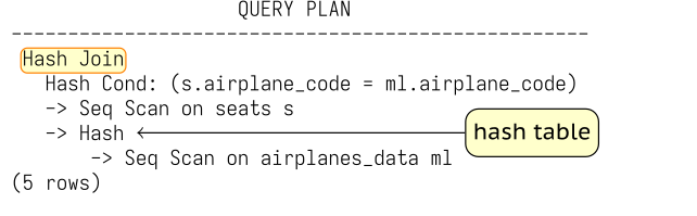
Hash Join first asks its Hash child to consume the inner input and build the hash table. It then reads the outer input and probes that table, returning matches as they are found.

Run the query:

EXPLAIN (analyze, costs off, timing off, buffers off)
SELECT *
FROM airplanes a
  JOIN seats s ON a.airplane_code = s.airplane_code;

                         QUERY PLAN
------------------------------------------------------------
 Hash Join (actual rows=1741.00 loops=1)
   Hash Cond: (s.airplane_code = ml.airplane_code)
   -> Seq Scan on seats s (actual rows=1741.00 loops=1)
   -> Hash (actual rows=10.00 loops=1)
       Buckets: 1024  Batches: 1  Memory Usage: 10kB
       -> Seq Scan on airplanes_data ml (actual rows=10....
 Planning Time: 0.047 ms
 Execution Time: 1.255 ms
(8 rows)

The hash table fits in memory. It uses 1024 buckets and about 10 kB. The planner chose the much smaller airplanes_data input for the build side.

The planner chose the much smaller airplanes_data input for the build side.

Multi-Batch Hash Join

If the planner estimates that the hash table will not fit in the memory of size work_mem × hash_mem_multiplier, the inner input is divided into batches, each of which is processed separately. The number of batches, like the number of buckets, is always a power of two; the batch number is determined by bits of the hash value. Rows that can match each other always belong to the same batch. Ideally, each batch contains approximately the same number of rows, but if values in the rows repeat, skew is possible.

When planning a query, the minimum required number of batches is calculated in advance so that the hash table for each individual batch fits in memory. This number is not reduced even if the planner’s estimate turns out to be pessimistic, but can be increased dynamically as needed.

First, PostgreSQL reads the inner input and builds the hash table. Rows belonging to the first batch remain in memory. Rows belonging to other batches are written to separate temporary files.

Then PostgreSQL reads the outer input. Rows belonging to the first batch are immediately matched against the first batch of the hash table, which resides in memory. Rows belonging to other batches are written to separate temporary files. Thus, with N batches, up to $2(N-1)$ temporary files are used; there may be fewer if some batches are empty.

Disk space used by temporary files in a session is limited by the value of temp_file_limit; temporary tables are not included in this limit.

After that, the memory occupied by the hash table is released. At this point the join already has a partial result for the first batch.

PostgreSQL then processes the batches saved on disk one by one. It loads the inner rows of a batch from its temporary file into the hash table, reads the matching outer rows from another temporary file, and joins them. The temporary files that have been processed are removed. The procedure repeats until all batches have been joined.

Join bookings and tickets, both large tables:

EXPLAIN (analyze, costs off, timing off, summary off)
SELECT *
FROM bookings b
  JOIN tickets t ON b.book_ref = t.book_ref;

                         QUERY PLAN
------------------------------------------------------------
 Hash Join (actual rows=5598473.00 loops=1)
   Hash Cond: (t.book_ref = b.book_ref)
   Buffers: shared hit=15839 read=57833 written=2, temp
   read=60337 written=60337
   -> Seq Scan on tickets t (actual rows=5598473.00 loop...
       Buffers: shared read=57816 written=2
   -> Hash (actual rows=2486710.00 loops=1)
       Buckets: 131072  Batches: 32  Memory Usage: 5155kB
       Buffers: shared hit=15839 read=17, temp
       written=12364
       -> Seq Scan on bookings b (actual rows=2486710.00...
           Buffers: shared hit=15839 read=17
 Planning:
   Buffers: shared hit=34 read=14
(14 rows)

The hash join uses 32 batches. The Hash node spills build-side data, while the Hash Join node also reads and writes temporary data as the batches are processed.

Now return only one column:

EXPLAIN (analyze, costs off, timing off, summary off)
SELECT b.book_ref
FROM bookings b
  JOIN tickets t ON b.book_ref = t.book_ref;
                         QUERY PLAN
------------------------------------------------------------
 Hash Join (actual rows=5598473.00 loops=1)
   Hash Cond: (t.book_ref = b.book_ref)
   Buffers: shared hit=15950 read=57722, temp read=25850
   written=25850
   -> Seq Scan on tickets t (actual rows=5598473.00 loop...
       Buffers: shared hit=94 read=57722
   -> Hash (actual rows=2486710.00 loops=1)
       Buckets: 262144  Batches: 32  Memory Usage: 5002kB
       Buffers: shared hit=15856, temp written=7927
       -> Seq Scan on bookings b (actual rows=2486710.00...
           Buffers: shared hit=15856
 Planning:
   Buffers: shared hit=18
(13 rows)

Memory consumption decreased, since the hash table now contains only one field (instead of the three that make up a row of the bookings table).

It is therefore important that:

• Only the fields that are actually needed are placed in the hash table

• The hash table is built on the smaller input

The first is the query author’s responsibility; the second, the planner’s.

Execution Cost

With a good hash distribution and an in-memory table, the expected amount of basic build-and-probe work is roughly proportional to $N+M$ for the two input sizes.

However, the hash table has to be built before the join can start, so for a small number of rows a nested loop is more efficient.

Hash join, combined with full table scans, is typical of OLAP queries that process many rows, where overall throughput is more important than response time.

Parallel Hash Join

Unlike other join methods, hash join not only can participate in parallel plans but also has an efficient parallel-aware algorithm. It parallelizes both phases of the join: building the hash table from the inner input and probing it with rows from the outer input. It is controlled by enable_parallel_hash and is enabled by default.

The memory budget is work_mem × hash_mem_multiplier × number of processes in this case. All processes can help scan the inner input and build one shared hash table. Once the build phase is complete, they cooperatively scan the outer input and probe that shared table.

Increase the amount of memory available to each process for building the hash table and run an aggregate query:

SET work_mem = '32MB';
EXPLAIN (analyze, costs off, timing off, buffers off)
SELECT count(*)
FROM bookings b
  JOIN tickets t ON b.book_ref = t.book_ref;
                         QUERY PLAN
------------------------------------------------------------
 Finalize Aggregate (actual rows=1.00 loops=1)
   -> Gather (actual rows=3.00 loops=1)
       Workers Planned: 2
       Workers Launched: 2
       -> Partial Aggregate (actual rows=1.00 loops=3)
           -> Parallel Hash Join (actual rows=1866157.67...
               Hash Cond: (t.book_ref = b.book_ref)
               -> Parallel Seq Scan on tickets t (actual...
               -> Parallel Hash (actual rows=828903.33 l...
                   Buckets: 4194304  Batches: 1  Memory
                   Usage: 130080kB
                   -> Parallel Seq Scan on bookings b (a...
 Planning Time: 0.161 ms
 Execution Time: 625.430 ms
(14 rows)

Note that the allocated memory exceeds the budget of one process: work_mem × hash_mem_multiplier = 64 MB in this example. Batches: 1 shows that the join stayed single-batch.

If the combined memory available to the parallel processes is still not enough for the whole hash table, PostgreSQL uses a multi-batch parallel algorithm.

First, the processes read the inner input in parallel, divide it into batches, and write the batches to temporary files. Unlike the serial algorithm, all batches, including the first one, are written to disk: each process reads only part of the inner input, so no process has a complete batch by itself.

After that, the outer input is also read in parallel, divided into batches, and written to temporary files. After the outer input has been read, there are 2N temporary files for N batches: one inner and one outer file per batch.

Each process then chooses an unprocessed batch, loads its inner rows into a hash table, reads the corresponding outer rows, and performs the join. In the multi-batch algorithm, each process has its own hash table of size work_mem × hash_mem_multiplier, but these tables reside in shared memory, meaning every parallel worker process can access each table.

When a process finishes one batch, it chooses another. If no unprocessed batches remain, a free process can help with a batch that another process is still processing, because the hash tables are in shared memory.

Using several smaller hash tables in this way makes coordination simpler and reduces synchronization overhead compared with having all processes work with one large shared hash table.

Reduce the memory setting:

SET work_mem = '16MB';

Run the same query:

EXPLAIN (analyze, costs off, timing off, buffers off)
SELECT count(*)
FROM bookings b
  JOIN tickets t ON b.book_ref = t.book_ref;
                         QUERY PLAN
------------------------------------------------------------
 Finalize Aggregate (actual rows=1.00 loops=1)
   -> Gather (actual rows=3.00 loops=1)
       Workers Planned: 2
       Workers Launched: 2
       -> Partial Aggregate (actual rows=1.00 loops=3)
           -> Parallel Hash Join (actual rows=1866157.67...
               Hash Cond: (t.book_ref = b.book_ref)
               -> Parallel Seq Scan on tickets t (actual...
               -> Parallel Hash (actual rows=828903.33 l...
                   Buckets: 1048576  Batches: 8  Memory
                   Usage: 20416kB
                   -> Parallel Seq Scan on bookings b (a...
 Planning Time: 0.112 ms
 Execution Time: 647.388 ms
(14 rows)

The join now uses eight batches.

4. Merge Join

The third main join method is merge join. Merge join exploits ordered inputs. If both row sets are ordered by compatible join keys, PostgreSQL can advance through them in key order and combine matching groups. The Gather Merge node works in a similar way: it merges already sorted streams into one sorted stream.

Sorting can be expensive—comparison sorting is typically $O(N \log N)$—but explicit sorting is not always necessary.

A B-tree index may already provide the required order, or an earlier plan node may preserve it.

A simplified mental model is that the input with the smaller current key advances until the keys catch up. When the keys are equal, matching rows are produced. Duplicate join keys complicate this picture. If one or both inputs contain several rows with the same key, PostgreSQL must produce all matching combinations for that key.

Consider a join in which both inputs are already available in the required order:

EXPLAIN (costs off) SELECT *
FROM tickets t
  JOIN segments tf ON tf.ticket_no = t.ticket_no
ORDER BY t.ticket_no;
                     QUERY PLAN
----------------------------------------------------
 Merge Join
   Merge Cond: (t.ticket_no = tf.ticket_no)
   -> Index Scan using tickets_pkey on tickets t
   -> Index Scan using segments_pkey on segments tf
(4 rows)

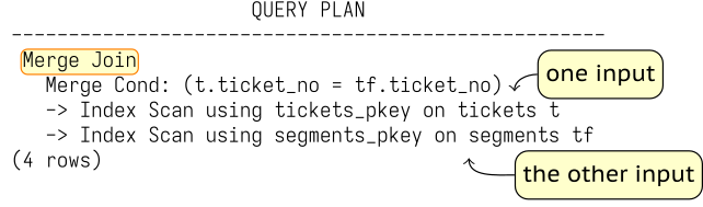
An important property of merge join is that it returns the join result in sorted order. In particular, the resulting row set can be used for another merge join without additional sorting or, as in this example, returned directly to the client.

In the following example, one Merge Join receives a sorted row set from another Merge Join:

EXPLAIN (costs off)
SELECT t.ticket_no, bp.flight_id, bp.seat_no
FROM tickets t
  JOIN segments tf ON t.ticket_no = tf.ticket_no
  JOIN boarding_passes bp ON bp.ticket_no = tf.ticket_no
                         AND bp.flight_id = tf.flight_id
ORDER BY t.ticket_no;

                         QUERY PLAN
------------------------------------------------------------
 Merge Join
   Merge Cond: (tf.ticket_no = t.ticket_no)
   -> Merge Join
       Merge Cond: ((tf.ticket_no = bp.ticket_no) AND (t...
       -> Index Only Scan using segments_pkey on segment...
       -> Index Scan using boarding_passes_pkey on board...
   -> Index Only Scan using tickets_pkey on tickets t
(7 rows)

Here segments are joined with boarding_passes, and tickets are then joined to this row set, which is already sorted by ticket number.

Execution Cost

If both inputs are already sorted on the merge keys, the basic merge pass is linear in the input sizes: $O(N+M)$. Unlike hash join, merge join does not need to build a hash table first. Merge join can therefore work successfully in both OLTP and OLAP queries.

However, if sorting is required, the cost becomes proportional to N log N, and for large data volumes this method will most likely lose to hash join.

Merge Join in Parallel Plans

Merge join can participate in parallel plans, but the Merge Join node itself is not a parallel-aware join algorithm in the same sense as Parallel Hash Join.

A common pattern is that one input is scanned in parallel, while each worker independently reads the complete other input far enough to find the matches it needs.

For large joins this duplicated work can make parallel hash join more attractive, because parallel hash was designed to share both the build and probe work.

Create an index that allows PostgreSQL to obtain tickets in book_ref order cheaply:

CREATE INDEX ON tickets(book_ref);

Now consider:

EXPLAIN (costs off) SELECT count(*)
FROM bookings b
  JOIN (
    SELECT book_ref FROM tickets GROUP BY book_ref
  ) t ON b.book_ref = t.book_ref;
                         QUERY PLAN
------------------------------------------------------------
 Finalize Aggregate
   -> Gather
       Workers Planned: 2
       -> Partial Aggregate
           -> Merge Join
               Merge Cond: (b.book_ref = tickets.book_ref)
               -> Parallel Index Only Scan using booking...
               -> Group
                   Group Key: tickets.book_ref
                   -> Index Only Scan using tickets_book...
(10 rows)

The scan of bookings_pkey is parallel. The grouped subquery on tickets, however, is read independently by each participating process that executes the merge join.

Remove the demonstration index:

DROP INDEX tickets_book_ref_idx;
DROP INDEX