2 Planning and Execution

1. Simple Query Protocol

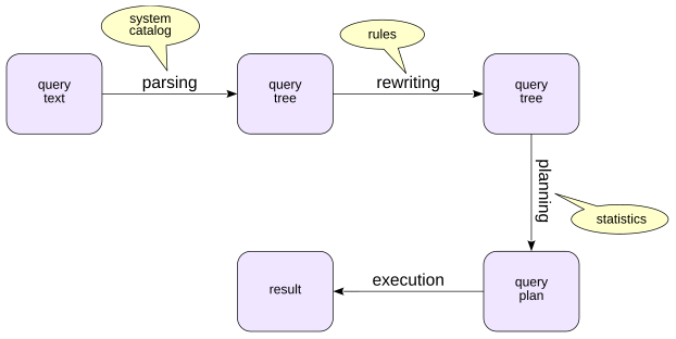
Start with the simplest case: what happens when you type, say, a SELECT command in psql. Query processing goes through several stages:

1. Parsing

2. Rewriting

3. Planning (optimization)

4. Execution

Parsing

Syntax analysis

The first step is parsing: PostgreSQL breaks the query text into tokens—identifiers, numbers, string literals, and so on—and checks that they form syntactically valid constructs.

Take a simple query:

SELECT  schemaname, tablename
FROM pg_tables
WHERE tableowner = 'postgres'
ORDER BY tablename;

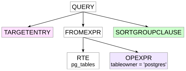
At this stage, the backend builds a parse tree in memory. The figure shows a simplified version of that tree. The colors indicate the approximate correspondence between parts of the query text and nodes of the tree.

RTE stands for Range Table Entry, a name that is not especially obvious from the outside. PostgreSQL uses RTEs internally for tables, subqueries, join results, and other row sets that can appear in an SQL query.

Semantic analysis

Next comes semantic analysis, called parse analysis in PostgreSQL. At this stage PostgreSQL determines which database objects the query refers to and whether the user has permission to access them.

SELECT  schemaname, tablename
FROM pg_tables
WHERE tableowner = 'postgres'
ORDER BY tablename;

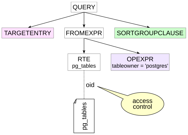
During parse analysis, PostgreSQL consults the system catalog. In our example, it resolves the name pg_tables to a particular view identified by an oid in the catalog. Access privileges on that view are checked as well.

Rewriting

The query is then rewritten according to rules.

An important special case is a view: a reference to a view is expanded into the query that defines the view. Strictly speaking, processing is not as neatly separated as this simplified sequence suggests, because the view definition also has to be parsed and analyzed.

For our example, the result can be pictured approximately like this:

SELECT  schemaname, tablename
FROM (
  SELECT ...
  FROM pg_class c
    LEFT JOIN pg_namespace n
      ON n.oid = c.relnamespace
    LEFT JOIN pg_tablespace t
      ON t.oid = c.reltablespace
  WHERE c.relkind = 'r'::"char"
)
WHERE tableowner = 'postgres'
ORDER BY tablename;

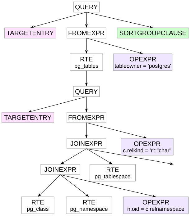
The SQL shown here is only an illustration. Rewriting operates on the query tree, not by substituting SQL text. In the tree, nodes corresponding to the view query are attached under the RTE for pg_tables.

Planning

PostgreSQL then plans the query.

The planner considers different ways to execute the query and estimates their costs using a mathematical model that operates on information about the data, called statistics. The candidate with the lowest estimated cost is represented as a plan tree.

A fragment of the plan for our example looks like this:

Sort
  Sort Key: c.relname
  ->  Nested Loop Left Join
        Join Filter: (n.oid = c.relnamespace)
        ->  Seq Scan on pg_class c
              Filter: ((relkind = 'r'::"char") AND pg_ge...
        ->  Seq Scan on pg_namespace n

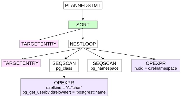
Seq Scan reads rows from a table, while Nested Loop joins two row sets. The textual representation in the figure is the form produced by the EXPLAIN command. We will discuss access methods and join methods in detail in later chapters.

Notice that only two of the original three tables remain: the planner has determined that one table is not needed to produce the result and has removed it from the plan.

Execution

Finally, the executor runs the selected plan and returns the result to the client.

The plan tree works as a pipeline. In the figure below it is redrawn to show only the essential structure.

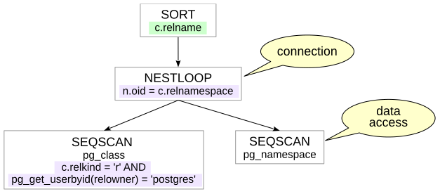
Execution starts at the root of the tree. The root node—in our case, Sort—requests data from its child. Once it has the data it needs, it performs its operation and returns rows upward, eventually to the client.

Nodes such as Nested Loop combine data from different sources. A join node requests rows from its two children, compares them according to the join condition, and returns matching pairs to its parent. The lower Seq Scan nodes fetch rows from the corresponding tables and pass them upward to the join.

Some nodes cannot return any result until they have consumed all the input they need. A regular sort is an example: it must see its input before it can determine the sorted order.

Other nodes can return rows as they arrive. A table scan, for example, can normally produce rows while it is still reading the table. This can make it possible to return the first part of a result quickly—for example, when an application displays data page by page. PostgreSQL documentation describes this executor mechanism as a demand-pull pipeline: a parent asks a child for the next row, and the request propagates down the plan tree.

2. Extended Query Protocol

By default, a client uses the simple query protocol: it sends an SQL statement to the server and, for a SELECT or a command with RETURNING, receives the result rows.

For example:

SELECT model FROM airplanes WHERE airplane_code = '77W';
      model
------------------
 Boeing 777-300ER
(1 row)

With the simple query protocol, every query goes through all of the processing stages described above, even if the same query is executed repeatedly.

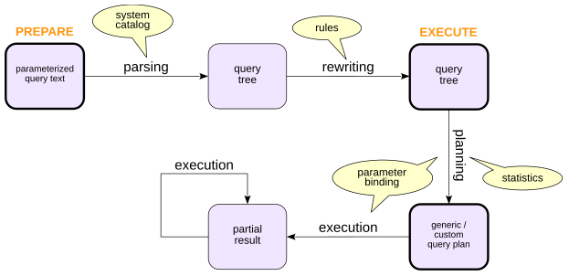
PostgreSQL also provides the extended query protocol, which separates query processing into more explicit steps. In practice, this makes it possible to prepare statements and use cursors.

Prepared Statements

To prepare a statement, the client sends the server a query, possibly containing parameters. The server parses, analyzes, and rewrites the query and retains the prepared statement state in the backend process.

To execute the prepared statement, the client supplies the values for its parameters. PostgreSQL can then build a custom plan that takes those particular values into account and execute it.

Preparing a statement avoids repeating parsing, analysis, and rewriting when the same statement is executed many times in one session.

If a statement has no parameters, there is no benefit in re-planning it for each execution, so PostgreSQL can reuse a generic plan.

If the statement does have parameters, PostgreSQL initially has the option of using custom plans and may later switch to a generic plan when it estimates that the generic plan is not significantly worse on average. We will return to that decision in Chapter VI, “Statistics.”

Prepared statements are also an important way to avoid SQL injection: values from an untrusted source can be sent separately as parameters instead of being concatenated into SQL text. This protection applies to values passed as parameters; dynamic SQL structure such as table or column names still has to be constructed safely.

Prepare a parameterized statement:

PREPARE model(varchar) AS
  SELECT model
  FROM airplanes
  WHERE airplane_code = $1;
PREPARE

Execute it by name:

EXECUTE model('CR7');
       model
-------------------
 Bombardier CRJ700
(1 row)

At execution time, the parameter value is bound, the statement is planned as needed, and then executed.

Prepared statements can be inspected through the pg_prepared_statements view:

SELECT * FROM pg_prepared_statements \gx
-[ RECORD 1 ]---+------------------------------
name            | model
statement       | PREPARE model(varchar) AS    +
                |   SELECT model               +
                |   FROM airplanes             +
                |   WHERE airplane_code = $1;
prepare_time    | 2026-09-25 17:14:48.990998+03
parameter_types | {"character varying"}
result_types    | {text}
from_sql        | t

executions with a generic plan

generic_plans   | 0
custom_plans    | 1

executions with custom plans

The last two columns show how many times the statement has used generic and custom plans. When a prepared statement is no longer needed, it can be removed with DEALLOCATE.

PREPARE, EXECUTE, and DEALLOCATE are SQL commands. Other programming languages expose the same idea differently, but database drivers ultimately use the same client/server protocol.

Cursors

Cursors make it possible to retrieve a query result incrementally instead of receiving all rows at once. They are common because applications are usually written in imperative languages and often process result sets iteratively.

Information about an open cursor is kept in the backend process.

Declare a cursor in SQL and fetch the first row. A cursor normally lives inside a transaction:

BEGIN;
BEGIN
DECLARE c CURSOR FOR SELECT * FROM airplanes;
DECLARE CURSOR
FETCH c;
 airplane_code |      model      | range | speed
---------------+-----------------+-------+-------
 32N           | Aerobus A320neo |  6500 |   830
(1 row)

Fetch the second row (the cursor will be closed automatically when the transaction ends):

FETCH c;
 airplane_code |        model        | range | speed
---------------+---------------------+-------+-------
 339           | Aerobus A330-900neo | 13300 |   870
(1 row)
COMMIT;
COMMIT

Database APIs provide ways to determine whether more result data remains, so an application can fetch from a cursor in a loop.

3. A Closer Look at Planning

Planning deserves a closer look because it is both central to query performance and one of the more complicated stages of query processing.

The Planning Process

The planner explores alternative execution plans, estimates their costs, and chooses the cheapest plan it finds.

A plan node’s cost depends on the operation being performed and on properties of the data it processes. Reading rows sequentially from a table obviously has a different cost model from fetching them through an index, and the amount of data being processed matters greatly.

Two concepts are especially important when estimating data volume:

• Cardinality: the estimated number of rows produced by a node

• Selectivity: the fraction of input rows that satisfy a condition, or predicate

Estimating selectivity and cardinality requires information about the data: table sizes, value distributions in columns, and so on. In practice, this brings us to statistics. PostgreSQL collects and refreshes statistics through autovacuum’s auto-analyze work and through the ANALYZE command. Cardinality errors are among the most important causes of poor plans.

They can come from insufficient statistics, from correlations that the available statistics do not describe, from expressions for which useful statistics are unavailable, or from limitations in the planner’s estimation models. Even a correct cardinality estimate does not guarantee a perfect cost estimate—the cost model and its parameters are approximations—but cardinality is a major input to almost every subsequent planning decision.

Cardinality Estimation

Cardinality estimation is recursive. To estimate the cardinality of a node, PostgreSQL first estimates the cardinalities of its children, then uses the node type and its predicates to estimate how many rows the node itself will produce.

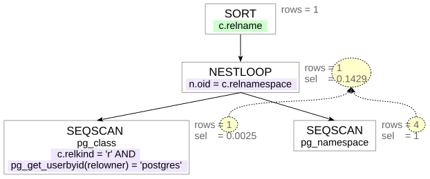
The process starts at leaf nodes, where access methods read data. Estimating them requires the size of the relation and the selectivity of its predicates. Later chapters show where those estimates come from.

Suppose for the moment that we can estimate the selectivity of simple predicates. Compound predicates can then be approximated with formulas such as

These formulas assume that conditions x and y are independent. If the predicates are correlated, the estimate can be wrong. PostgreSQL’s extended statistics can improve some of these cases.

Next come joins. We already have cardinality estimates for the two input row sets, so we also need an estimate of the join condition selectivity. We will postpone the details and return to concrete examples later.

Other nodes can be treated in a similar way—for example, aggregation. A sort normally preserves cardinality, while other operations may change it.

An estimation error introduced low in the plan tree propagates upward. It can become amplified as more operators depend on the incorrect estimate and can eventually lead the planner to choose a poor plan.

Cost Estimation

Cost estimation is recursive as well. To estimate the cost of a plan subtree, PostgreSQL starts with the costs of its child nodes and adds the cost of the operation performed by the current node.

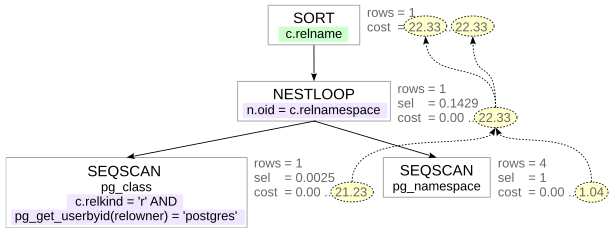
The cost of a node is computed from the planner’s mathematical model using the cardinality and other properties estimated for that node.

EXPLAIN shows two cost components: startup cost defines the estimated work that must be done before the node can begin producing rows, and total cost defines the estimated cost of producing all rows.

Some operations require little or no startup work. Other operations have to do substantial work before returning the first row.

A regular sort, for example, must consume the input that it needs to sort before it can emit sorted output. Such a node has a nonzero startup cost, which has to be paid even when the consumer needs only a small part of the final result.

It is important to understand that cost reflects the planner’s estimate and may not correlate with actual execution time. Cost can be thought of as being expressed in arbitrary units that mean nothing by themselves. It is needed only so that the planner can compare different plans for the same query.

Choosing the Best Plan

The optimizer tries to find the best plan without spending unreasonable time planning.

For joins, PostgreSQL normally uses dynamic programming to build larger join relations from smaller ones while discarding alternatives that cannot win under the planner’s criteria. As the number of relations grows, exhaustive consideration of join orders becomes too expensive. PostgreSQL can reduce the number of plans it considers, either by considering only some pairwise join alternatives or by switching to the Genetic Query Optimizer (GEQO). This creates another possible source of a poor plan: not an incorrect cost estimate, but the fact that the best plan was never considered. In such cases the query author can sometimes help by constraining the join order.

What counts as the ”best” plan? For an ordinary query, PostgreSQL normally optimizes for obtaining the complete result, so total cost dominates.

With cursors, however, getting the first rows quickly can matter more. The parameter cursor_tuple_fraction (default 0.1) tells the planner what fraction of the cursor’s rows is expected to be retrieved. A smaller value gives startup cost more influence relative to total cost.

Viewing a Query Plan

EXPLAIN displays a query plan. It is the indispensable tool for query performance work, and learning to read it well is essential. Here is the plan for the query we used above:

EXPLAIN SELECT schemaname, tablename
FROM pg_tables
WHERE tableowner = 'postgres'
ORDER BY tablename;
                         QUERY PLAN
------------------------------------------------------------
 Sort  (cost=22.36..22.37 rows=1 width=128)
   Sort Key: c.relname
   -> Nested Loop Left Join
       (cost=0.00..22.35 rows=1 width=128)
       Join Filter: (n.oid = c.relnamespace)
       -> Seq Scan on pg_class c
           (cost=0.00..21.26 rows=1 width=72)
           Filter: ((relkind = ANY ('{r,p}'::"char"[])) ...
       -> Seq Scan on pg_namespace n
           (cost=0.00..1.04 rows=4 width=68)
(10 rows)

Adding analyze makes PostgreSQL execute the query and show actual execution statistics as well as estimates:

EXPLAIN (analyze, buffers off) SELECT schemaname, tablename
FROM pg_tables
WHERE tableowner = 'postgres'
ORDER BY tablename;
                         QUERY PLAN
------------------------------------------------------------
 Sort  (cost=22.36..22.37 rows=1 width=128)
   (actual time=0.101..0.103 rows=77.00 loops=1)
   Sort Key: c.relname
   Sort Method: quicksort  Memory: 35kB
   -> Nested Loop Left Join
       (cost=0.00..22.35 rows=1 width=128)
       (actual time=0.009..0.080 rows=77.00 loops=1)
       Join Filter: (n.oid = c.relnamespace)
       Rows Removed by Join Filter: 112
       -> Seq Scan on pg_class c
           (cost=0.00..21.26 rows=1 width=72)
           (actual time=0.006..0.039 rows=77.00 loops=1)
           Filter: ((relkind = ANY ('{r,p}'::"char"[])) ...
           Rows Removed by Filter: 382
       -> Seq Scan on pg_namespace n
           (cost=0.00..1.04 rows=4 width=68)
           (actual time=0.000..0.000 rows=2.45 loops=77)
 Planning Time: 0.080 ms
 Execution Time: 0.113 ms
(19 rows)

Be careful with EXPLAIN ANALYZE on statements that modify data: the statement is actually executed.

Collecting timing information for every plan node can noticeably slow a query on some platforms. If you do not need per-node timing, disable it with timing off.

Referenced resources

• www.postgresql.org/docs/18/protocol-flow
• www.postgresql.org/docs/18/query-path
• www.postgresql.org/docs/18/using-explain